Understanding Muse Spark Open

A week ago this showed up on my feed:

We’re launching a $100,000 challenge to see who can make Muse Spark run fastest: openkernelchallenge.dev
— Daniel Gross (@danielgross) October 22, 2026

The model it refers to had come out only a week earlier. On October 15 Meta released Muse Spark Open, the full-size member of its Muse series, with open weights.

The challenge#

A model this size doesn’t run on one GPU. It runs on a node of eight H200s, and the question the challenge asks is how fast can you make it go? There are two tracks.

The kernel track takes the model apart into five pieces and asks you to make each one faster than SGLang, the inference engine Meta ships it with. Each piece is one problem, and each problem runs on a single H200:

The dense projections (plain matrix multiplies).
Attention during decoding.
The routed experts, the part that holds 97% of the parameters.
A whole decoder layer while decoding.
A whole decoder layer during prefill, when the model reads the prompt.

You submit a Python file. The judge runs it on an H200, checks that it gives the same answers as the reference, and times it against SGLang. A score of 1.00× means you tied; anything above means you won some time back. Kernel submissions close on November 4.

The serving track opens the day after, on November 5, and is where the money is: you patch SGLang itself and the judge runs the whole model on the whole node.

Diving into Muse#

The problem statement for the prefill layer says “most of the time goes to the routed experts.” I copied SGLang’s baseline, ran the judge’s profiler, and it agreed: about 65% of the time is inside the experts.

And then I realized I couldn’t picture what an expert does to a token. I could read the formula in the spec. I could see the shapes of the weight matrices. But I had no mental image of a token entering the layer, getting routed, being multiplied by a 4-bit matrix and coming out the other side. Making that faster without understanding it felt like running blindfloded.

So, this seemed like a great excuse to get to understand the model, piece by piece.

The overview#

Before opening anything, here is an overview of the model’s architecture.

A prompt comes in through one of three doors. Text goes through a tokenizer; images and video through a perception encoder; audio through an audio encoder. Whatever the door, what comes out is the same thing: a list of tokens, each one a vector dim 8,192. That list, $[T, 8192]$ , is the shape that travels through everything below.

Then we get 62 layers, each layer performs Attention, where the token looks at the tokens before it and pulls information from them and mixture of experts, where the token gets processed on its own. A router scores 256 small networks, picks the 8 best, and the token runs through those 8 only. That’s why we get onnly 42B active params although the model has a total of 816B. This is the interesting part of the model for the challenge, its the one that takes the longest and has lots of room for optimization.

You may also notice that between the two there is a residual stream: the orange line on the left of the figure. Each block adds its result to it instead of replacing it, an idea from ResNet that lets a layer do nothing when nothing is the right thing to do.

Left: the model, as Meta draws it. Right: one of the 62 layers. The side arrows are the residual: each block's output is mixed back into it through a learned gate rather than a plain sum.

Where the parameters are. Area is proportional to the number of parameters; the experts hold 97% of them. Counts from the model card's dimensions.

Also, another interesting thing is that not all 62 layers do the same. 46 of them attend only to a window of the last 2,048 tokens and the other 16 attend to the whole context. Those are alternated in a fixed pattern of four: sliding, full, sliding, sliding.

The 62 layers in order. The pattern repeats every four: sliding, full, sliding, sliding.

Overview of one layer#

Lets look inside on of the 62 layers. If we see it as a black box, a layer is a function that takes a list of vectors and returns a list of vectors of the same shape. The input is the residual stream $s$ : one vector of 8,192 numbers per token, and the output is the same shape. The layer edits the stream twice: once with attention and once with the mixture of experts.

One of the 62 layers. The orange path is the residual stream; it is never replaced, only mixed with each branch's output through a learned gate.

1 / 8

The stream comes in

\htmlClass{hs}{s} \in \mathbb{R}^{T \times 8192}

The residual stream from the previous layer, one vector of 8,192 numbers per token. We follow one of those tokens.

Use ‹ › or the arrow keys, or click a box in the figure.

Before a branch sees the stream it gets normalized:

\text{rms}(x) = \frac{x}{\sqrt{\tfrac{1}{d}\sum_i x_i^2 + \varepsilon}}, \qquad h = \text{rms}(s) \cdot (1 + w)

RMSNorm divides the vector by its root-mean-square, so whatever scale $s$ has drifted to, the branch always receives a vector of size about $\sqrt{d}$ . The learned $w$ (one per dimension) lets the model scale some dimensions up or down on the way in. Writing it as $1 + w$ means the untrained norm is the identity, cause it starts with $w = 0$ . $\varepsilon$ is there just for numerical stability, and $d$ is the dimension of the vector, 8,192.

This is called pre-norm, the norm is on the branch, not on the trunk. The stream itself is never normalized in place.

Attention, then a gate#

The normalized $h$ goes through attention and comes back as $a$ , also $[T, 8192]$ . In a plain transformer the next step is $s \leftarrow s + a$ . Muse does something slightly different:

s \leftarrow \alpha_1 \cdot s + \beta_1 \cdot \text{rms}(a)

There are two differences. First, $a$ gets normalized before being added, so the attention output always has the same size no matter what came out of it. Second, instead of a plain sum we have a weighted sum: $\alpha_1$ says how much of the old $s$ we keep and $\beta_1$ how much of the new information we add. Both are learned, and there is one value per dimension, so each of the 8,192 dimensions has its own mix. Meta calls this a learned residual gate. The reason is that with a plain sum $s$ gets bigger at every layer, and after 62 layers it can grow a lot. With the gate it stays in a fixed range.

Experts, then another gate#

The second half works exactly the same way. We normalize $s$ again, this time with its own $w$ , and send the result $h$ through the mixture of experts. What comes back is $f$ , again $[T, 8192]$ , and it gets mixed into the stream with a second gate:

s \leftarrow \alpha_2 \cdot s + \beta_2 \cdot \text{rms}(f)

$\alpha_2$ and $\beta_2$ are a different pair of learned values, one per dimension, like before. After this $s$ has been edited twice, once by attention and once by the experts, and it goes into the next layer.

What differs between the 62#

All 62 layers have this same structure, what changes are the weights: each layer has its own $w$ , $\alpha$ , $\beta$ , its own attention matrices and its own 256 experts. The only difference in structure is the one we saw before: in 46 of the layers attention is sliding and in 16 it is full. Everything else is the same, and every layer has a mixture of experts, there are no dense layers.

Inside an Attention Block#

Where attention sits in the layer: it reads h, the normalized stream, and returns a, which the gate mixes back into the stream.

Attention in Muse is the one you already know, with a few changes on top. Written out, the block is this:

The attention block. The numbered parts are where Muse differs from textbook attention; each number links to its section below.

If the mechanism itself is new to you, Jay Alammar’s visual guide to attention is a good place to start.

One matrix, four pieces#

The first thing is that $h$ gets multiplied by a single matrix $W_{qkvg}$ and the result is split into four pieces: the queries $q$ , the keys $k$ , the values $v$ and a fourth one, $g$ , that we will get to at the end. $q$ has 128 heads and $k$ and $v$ have 16 each, all of 64 numbers. $128 \times 64 = 8192$ , so the queries keep the full width of the model.

The same block with the size of everything that flows through it, for one token. The two matrices are drawn as grids; the KV cache grows by one row per token.

Inside × W_qkvgᵀ, on a small example: 6 tokens of 16 numbers times a 16 × 40 matrix. The tokens are on the left face, the matrix on the top face, the result in front. Each result number is where a row of the left meets a column of the top: 16 products, added up along the line.

128 query heads, 16 key and value heads#

Having 128 query heads but only 16 key and value heads is called grouped-query attention: every 8 query heads share the same $k$ and $v$ . The reason is memory. The keys and values of every past token have to be stored (that is the KV cache), and that cost depends on the number of $k$ and $v$ heads, not $q$ heads. With 16 instead of 128, the cache is 8 times smaller. Muse also stores it in FP8, one byte per number. More on GQA in the paper that introduced it.

The same block for one group of heads: 8 q heads (8 thin lines), one k head and one v head they all share. Muse has 16 of these groups.

QK-norm#

Then $q$ and $k$ get normalized before the dot product. This is called QK-norm. It keeps $q k^T$ in a bounded range, so the softmax never gets a huge score that makes it collapse onto one token. It costs almost nothing and most recent models do it.

QK-norm. Each head of q and k is a vector, drawn here as an arrow whose length is its size. Dividing every head by its size puts all of them on the same circle: their directions stay, their sizes become equal, so no single score can grow out of range.

Sliding and full layers#

The mask is causal in every layer, a token only sees the ones before it. In the sliding layers it also cuts everything further back than 2,048 tokens. That is the only difference between a sliding and a full layer.

Which keys each query can see. Row i is token i asking; a filled cell means it can look at that token. In the real model the window is 2,048, not 4.

RoPE, the rotation that tells attention how far apart two tokens are, is only applied in the 46 sliding layers. In the 16 full layers it is not applied at all, so those layers have no idea of position, only of content. Mixing layers with and without RoPE this way was proposed by Cohere, and Llama 4 does it too: the sliding layers already know about position, and layers without positions cope better with lengths longer than the ones they were trained on.

q at position 2 k at position 5

RoPE on one head of q and one of k, 8 numbers each here (64 in Muse). Each pair of numbers is an arrow, and RoPE turns it by the token's position times that pair's speed: the numbers change, the arrow's length doesn't. Below, how much each pair adds to q · k. Shift both tokens and nothing below moves: only the gap between them counts.

The output gate#

And finally $g$ . It has the same shape as the attention output, 128 heads of 64. The output of each head gets normalized and then multiplied, number by number, by $\sigma(g)$ , a sigmoid, so a value between 0 and 1. For every token, every head can turn its own output down, all the way to zero. In a normal transformer a head can’t say “I have nothing to add for this token”, it has to attend to something, usually the first token, and that is where attention sinks come from. With the gate it can just output zero. After the gate, $W_o$ brings the 8,192 numbers back into the shape of the stream, and that is $a$ .

The output gate. Each head arrives from × v and passes through one fader per number. g, which comes straight out of W_qkvg, sets every fader between 0 and 1 through σ. Head 1 passes almost untouched, head 2 is turned down, head 3 has nothing to add for this token and is switched off, and head 4 keeps all but one number. What is left goes on to W_o.

The KV cache at a million tokens#

Every token that goes through attention leaves its $k$ and $v$ in the KV cache of every layer, so that the tokens after it can read them without computing them again. Muse can read up to a million tokens, so this cache is the biggest memory cost of running it.

The KV cache of one layer and one key/value head: a row of k and a row of v for every token so far. The new token writes its row at the bottom, its q is compared with every k, and the next token will add one more row.

Done the plain way, with one key and value head for each of the 128 query heads, 64 numbers each in BF16, the cache takes $62 \times 128 \times 64 \times 2 \times 2$ bytes, almost 2 MB per token. At a million tokens that is about 2 TB, more than the memory of all 8 GPUs together. Muse makes it about 60 times smaller with choices we have already seen:

Grouped-query attention: 16 key and value heads instead of 128, 8 times smaller.
FP8: one byte per number instead of two, 2 times smaller.
Sliding layers: 46 of the 62 layers only keep the last 2,048 tokens, so only the 16 full layers grow with the conversation, almost 4 times smaller.
The 8 GPUs split the 16 heads between them, 2 each, so each GPU holds an eighth.

In the end it is about 33 KB per token, about 35 GB at a million tokens, and about 4 GB on each GPU, next to the 141 GB an H200 has.

context:

The KV cache at each step, on a log scale: from the plain design to what one GPU holds, against the memory of one H200 and of the whole node. Switch the context length: below 2,048 tokens the sliding window doesn't help yet, at a million it is what makes the difference.

Inside the Mixture of Experts#

The second half of the layer: the normalized stream goes into the mixture of experts, and what comes out, f, is mixed back into the stream by the second gate.

The second half of every layer is the mixture of experts. In a dense model this half would be one big feed-forward network, and every token would be multiplied by all of its weights. A mixture of experts splits it into many small networks, the experts, and each token only goes through a few of them. That is how Muse has 816B parameters but only uses about 42B for each token, and why this half is where most of Muse is: 799B of its 816B parameters, and in the challenge about two thirds of the time of a layer.

The mixture-of-experts block. The numbered parts are where Muse differs from a typical MoE; each number links to its section below.

The router reads the whole token, in FP32#

The router decides which 8 experts each token goes to, and it is just one matrix multiplication:

s = h \, W_r

$h$ is the token, 8,192 numbers, and $W_r$ is the router’s matrix, with 8,192 rows and 256 columns, one column per expert. The result $s$ has 256 numbers, one score per expert. Each score is the dot product of $h$ with that expert’s column, so it is high when the token points in the same direction as the column. The 8 highest scores pick the experts, and those same 8 scores are turned into the weights used at the end to mix the outputs of the 8 experts. Every layer has its own router, so a token can go to different experts in every layer.

The router is one matrix multiplication. h, standing on the left, meets every column of W_r, one column per expert. Each score sits under its column and is h times that column: 8,192 products added up. The 8 highest scores pick the experts, and the same scores become the weights of their outputs at the end.

The matrix is small next to the experts: $8{,}192 \times 256 \approx 2.1\text{M}$ numbers per layer, against 50M in a single expert. In Muse the router reads $h$ at its full size, before the squeeze, and it works in FP32 while the rest of the layer is in BF16 or less. The vLLM recipe gives the reason: picking the wrong expert costs more than running a smaller one.

256 experts, 8 per token, no shared expert#

Each layer has 256 experts, and every token goes through 8 of them. Different tokens pick different experts, so all 256 get used, but each token only pays for 8. Many recent MoE models also have a shared expert that every token goes through: DeepSeek-V3 has one next to its 256 routed experts, and Llama 4 has one next to 16 or 128. Muse has none, so everything a token gets from this half of the layer comes from the 8 experts it picked. Having many small experts instead of a few big ones comes from DeepSeekMoE: there are about $4 \times 10^{14}$ ways to pick 8 out of 256, against 28 ways to pick the 2 out of 8 of Mixtral, so each token gets a much more specific mix.

Four tokens and the 8 experts each one picks, out of 256: different for every token, with nothing shared. DeepSeek-V3, on the right, also sends every token through one shared expert.

Inside one expert#

Each of the 8 experts is a small gated feed-forward network, the kind most recent models use, with three matrices of $4{,}096 \times 4{,}096$ : gate, up and down. Gate and up both read $x$ , the token after the squeeze. The result of gate goes through an activation function and multiplies the result of up number by number, and down takes that back to 4,096 numbers. In a dense model up takes the token to a bigger size, about 3 times the model’s width, which is where the name comes from. Here the middle is also 4,096 wide, so the three matrices are square and up doesn’t actually go up.

What is different is what comes after: the expert normalizes its output. Most MoE models don’t have this norm. It puts the 8 outputs on the same size, so how much each one counts is decided only by the router’s weight. That output, times the router’s weight for this expert, is what gets added up with the other 7.

One expert, with every step drawn as the vector it produces (10 cells stand for 4,096 numbers). Gate and up both read x. The gate's result, through the activation, sets one fader per number, and up's result passes through them: what is strong on the left and has its fader turned up stays strong on the right. Down brings it back to 4,096, the norm evens out its size, and the router's weight scales it before it is added to the other 7.

Go deeperHow a gated feed-forward network works4 figures · 5 min

Written out, the whole expert is one line:

y = W_{down}\,\big(\text{act}(W_{gate}\,x) \odot W_{up}\,x\big)

$x$ is the token after the squeeze (4,096 numbers). $W_{gate}$ , $W_{up}$ and $W_{down}$ are the three $4{,}096 \times 4{,}096$ matrices. $\text{act}$ is the activation, applied to every number on its own. $\odot$ means multiplying number by number. $y$ is what the expert gives back, before its norm.

The easiest way to read it is one middle number at a time. There are 4,096 of them, and we call each one a unit. Unit $i$ owns three things: row $i$ of $W_{gate}$ , row $i$ of $W_{up}$ and column $i$ of $W_{down}$ . For a token, the gate row times $x$ gives one number, and the activation turns it into the position of a fader. The up row times $x$ gives another number, positive or negative: a value. The value times the fader is what the unit lets through, its amount, and the unit adds column $i$ of $W_{down}$ , times that amount, to the output.

One unit, highlighted inside the three matrices of an expert: a row of gate, a row of up and a column of down. The gate row gives a fader position, the up row a value, their product is the amount, and the down column is what gets added to the output, times that amount.

Here it is with every number, on a token of 3 numbers instead of 4,096 and with 2 units instead of 4,096. The token is $x = [1,\ 0.5,\ -1]$ . For unit 1 the gate row gives $2 + 0 - 1 = 1$ , and the up row $1 + 1 + 0 = 2$ . Say the activation turns the 1 into a fader at 0.73 (the real activation isn’t public yet, this one is only to have numbers), so unit 1 lets through $0.73 \times 2 = 1.46$ . For unit 2 the gate row gives $-1.5$ , which becomes a fader at 0.18, and the up row gives 2 again, so it lets through $0.18 \times 2 = 0.36$ . Both units found the same amount of their feature, but unit 2’s gate says it matters less for this token, so it passes 5 times less. Then $y$ is unit 1’s column of down times 1.46, plus unit 2’s column times 0.36.

The tiny example with every number. Each result sits right next to the row that produced it. The two amounts, 1.46 and 0.36, scale the two columns of down, and adding them up gives y = [1.09, −1.10, 0.36].

With 4,096 units it is the same thing, just wider: $y$ is the sum of the 4,096 columns of $W_{down}$ , each one times what its unit let through. For a given token most units let through very little, so $y$ is mostly made of the few columns whose units fired. The three matrix multiplications in the expert figure above are these 4,096 units done all at once.

All the units of one expert at once (48 drawn instead of 4,096). The bars on top are what each unit let through; most are close to zero. Each column of down is drawn bright only if its unit let something through, and y is the sum of all the columns, each times its unit's amount.

The original transformer used a plain feed-forward network, $y = W_2\,\text{ReLU}(W_1\,x)$ , with two matrices. ReLU turns negatives into 0 and leaves positives as they are. There, a unit has only one row, so the same number decides whether the unit fires and how much it writes, and it can never write a negative amount. The gated version splits that in two: the gate row decides whether, and the up row decides how much and with what sign. That costs one more matrix, and it trains better.

What one unit writes, depending on what it reads. On the left, the plain version: one number goes in, and the amount is 0 or that same number. On the right, the gated version: the amount depends on two numbers from two different rows. With the fader closed (left half) nothing is written, whatever the value; with it open, the value goes through with its sign (orange positive, blue negative).

So each unit is a rule of the shape “if the gate’s pattern is there, add this column, scaled by how much of the up feature there is”, and this paper shows feed-forward layers working like that. One expert has 4,096 of these rules, a layer has $256 \times 4{,}096 \approx 1\text{M}$ , and the whole model about 65M. A token only uses the rules of its 8 experts in each layer, which is what the router decides.

Experts in a smaller space#

In most MoE models every expert reads the token at the model’s width and gives back a vector of the same width. Muse first multiplies $h$ by a matrix that squeezes it from 8,192 down to 4,096 numbers, runs the experts at that size, and after mixing their outputs brings the result back to 8,192 with a second matrix. These two matrices are shared by all the experts. So each expert has three $4{,}096 \times 4{,}096$ matrices, about 50M parameters, and $256 \times 62 \times 50\text{M} \approx 799\text{B}$ , the published number. At the model’s width every expert would be twice as big. What comes out of the second matrix is $f$ , the one the second gate of the layer mixes into the stream.

One expert, drawn to scale (inputs across, outputs down). Reading the token at the model's width, an expert needs three 8,192 × 4,096 matrices, and 256 × 62 of them would be 1.6T parameters. At 4,096 it needs three 4,096 × 4,096 matrices, and 256 × 62 of them are the 799B Meta publishes. The squeeze and the expand are paid once per layer.

Even at 799B the experts don’t fit: in BF16 they take 1.6 TB, more than the 1,128 GB of a node with 8 H200s. So Meta also publishes the weights in NVFP4, a 4-bit format where every 16 numbers share a small scale, about 4.5 bits per number, which brings the experts down to about 450 GB. NVIDIA’s introduction to NVFP4 explains how the format works. The H200 has no 4-bit math, so the weights are turned back into BF16 as they are read: the memory is saved, but the multiplications still happen in BF16.

The weights of all the experts in BF16 and in NVFP4, against the memory of a node with 8 H200s. Only the 4-bit version fits.

After the 62nd layer#

After the 62nd layer, only the last token matters. Its stream goes through the output layer, a matrix that turns its 8,192 numbers into one score for each of the 202,048 tokens of the vocabulary, and one of them is picked, like the “in” at the end of the overview figure. That token goes back in at the start, as the next one. Everything the earlier tokens left behind is already in the KV cache of every layer, so for the next step only the new token has to go through the 62 layers.

Running Muse on 8 GPUs#

Even in NVFP4 the experts take about 450 GB, and one H200 has 141 GB, so Muse runs on all 8 GPUs of the node, and every layer is split across them. Attention is split by heads: each GPU takes 2 of the 16 key and value heads and the 16 query heads that go with them, so each GPU also keeps its own part of the KV cache. The experts are split whole: each GPU keeps 32 of the 256.

32 experts per GPU#

The 8 experts of a token are usually on different GPUs. So the token is sent to every GPU that holds one of its experts, each of those GPUs runs it through that expert, and the outputs are sent back to be added up.

The 256 experts split over 8 GPUs, 32 each. The 8 experts one token picked are on 6 different GPUs, so the token has to visit all of them.

Tokens travel in batches#

Doing this one token at a time would be far too slow, so Muse never does it. When it reads a prompt, all the new tokens go through each layer together, and while it generates, the next token of many conversations goes through together. That group is a batch. In the challenge, a turn of an agentic coding conversation brings 753 new tokens, so a batch there is 753 tokens.

All the tokens of a batch go through the router first, and each one gets its 8 experts. Then they are grouped by expert: every expert collects the tokens that picked it and multiplies all of them at once, in a single matrix multiplication. The reason is memory: an expert’s weights have to be read every time it runs, and this way they are read once for all its tokens instead of once per token, and the trips between GPUs carry many tokens at once. At the end each token gets back the outputs of its 8 experts and adds them up, weighted by the router. An expert that no token picked does nothing in that batch.

A small batch: 6 tokens, 8 experts and 2 picks each (in a turn of the challenge, 753 tokens, 256 experts and 8 picks). Each token picks its experts, the tokens are grouped by expert so that each expert does one multiplication with all of its tokens, and the outputs go back to each token, where they are weighted and added up. Nobody picked E5 or E8, so they sit idle.

With 753 tokens and 8 picks each there are $753 \times 8 = 6{,}024$ picks, spread over 256 experts, so each expert gets about 24 tokens. Every time an expert’s weights are read, each of them is used about 24 times. Spread over the 8 GPUs, that is about $6{,}024 / 8 \approx 753$ picks per GPU, still about 24 for each of its experts.

When many tokens pick the same expert#

Those numbers are averages. The router picks experts by what each token is about, so some experts can end up much more popular than others. If many tokens of a batch pick experts that live on the same GPU, that GPU gets far more work than the rest, and the whole layer waits for it while the other seven are already done. That is why MoE models are trained to spread the tokens evenly, for example with the extra loss term that Switch Transformer adds, which penalizes the router when it sends too many tokens to the same experts.

The 753 new tokens of a turn make 6,024 picks, spread over the 8 GPUs. Balanced, every GPU gets about 753 and they all finish together. Unbalanced, GPU 1 holds the popular experts and gets 2,050, and the layer waits for it.

Why the experts take most of the time#

In the challenge the experts take about two thirds of the time of a layer. The first reason is that they have most of the math. In every layer a token is multiplied by about 690M weights, and 403M of them are in its 8 experts.

The weights one token is multiplied by in one layer, drawn to scale. Attention's two matrices are about a third; the 8 experts the token picked are more than half.

The second reason is less obvious. To run an expert, the GPU has to do two things: read the expert’s weights from memory, and do the multiplications with them. An H200 reads its memory, the HBM, at about 4.8 TB/s, and does about 989 trillion operations per second in BF16. The 4-bit weights of one expert are about 28 MB, so reading them takes $28\text{ MB} / 4.8\text{ TB/s} \approx 5.9$ µs, and it takes almost the same whether the expert got 1 token or 500. The math is different: each token is multiplied by the expert’s 50M weights, a multiplication and an addition for each, so 100M operations, and $100\text{M} / 989\text{T} \approx 0.1$ µs per token. A good kernel does both at the same time, so the expert takes as long as the slower of the two.

One expert, for the cases of the challenge. The memory lane (blue) reads the weights and always takes 5.9 µs; the math lane (orange) gets one slice per token. Both run at the same time, and the lane that finishes first sits idle (hatched) until the other is done. Below 58 tokens the math waits for the memory, above it the memory waits for the math.

In a turn each expert gets about 24 tokens, so the math is done in 2.4 µs and the GPU spends the rest of the 5.9 µs waiting for the weights. Both take the same time at about 58 tokens per expert. Above that the math decides, which is the case when four conversations come at once (about 94 tokens per expert) and in the first turn, which reads the prompt in chunks of 16,384 tokens (512 per expert). While generating, a single conversation gives each of its experts one token, and the GPU waits almost the whole time. This is also why the 4-bit weights matter for speed and not only for memory: in BF16, reading one expert would take about 21 µs instead of 5.9.

Go deeperThe same thing, as a roofline1 figure · 2 min

Another way to see it is to count how many operations the GPU gets to do for every byte of weights it reads. An H200 can do about 989 trillion operations per second and read about 4.8 TB per second, so it can do about 206 operations in the time it reads one byte. With 4-bit weights an expert does about 3.6 operations per byte for each of its tokens, so with 24 tokens it does about 85 per byte, below the 206, and the GPU waits on memory. The two meet at $206 / 3.6 \approx 58$ tokens, the same crossover as above. Drawn on a log scale, this is called a roofline.

For every byte of expert weights the GPU reads, how much math it gets to do, by how many tokens each expert gets (both on a log scale). Below the dashed line, about 206 operations per byte on an H200, the GPU waits on memory; above it, on the math. A turn of the challenge is below the line, four conversations at once and the first turn are above it, and generating is far below.

This is the interesting part of the model for the challenge. Each GPU holds 32 experts, so in a turn just reading their weights takes about $32 \times 5.9 \approx 190$ µs, and SGLang takes 757 µs. With four conversations the math alone takes about 310 µs, and SGLang takes 2,236 µs. So there is room for being 4 to 7 times faster.

The experts of one layer on one H200, as SGLang runs them today. The solid part is the floor, the slower of the two lanes: reading the weights on a turn, the math with four conversations at once. The hatched part is the time a better kernel could win back.

Back to the five problems#

With the whole model in view, the five problems of the kernel track are five cuts of the same layer. Each one runs on a single GPU of the eight, so it only gets that GPU’s part of the layer: 16 of the 128 query heads, 2 of the 16 key and value heads, and 32 of the 256 experts.

Four of them time Muse while it generates. Each step brings one new token for each conversation, with 1, 16 or 32 conversations at once and about 80K tokens of context each. SGLang’s default setup also uses speculative decoding: each conversation brings a draft of 8 guessed tokens, and Muse checks all 8 in one step, so a step can also carry 8, 128 or 256 tokens. Those six batches are what the four problems are timed with. The fifth problem is the one from the experts section: reading a turn of 753 tokens, four conversations at once, and the first turn in chunks of 16,384.

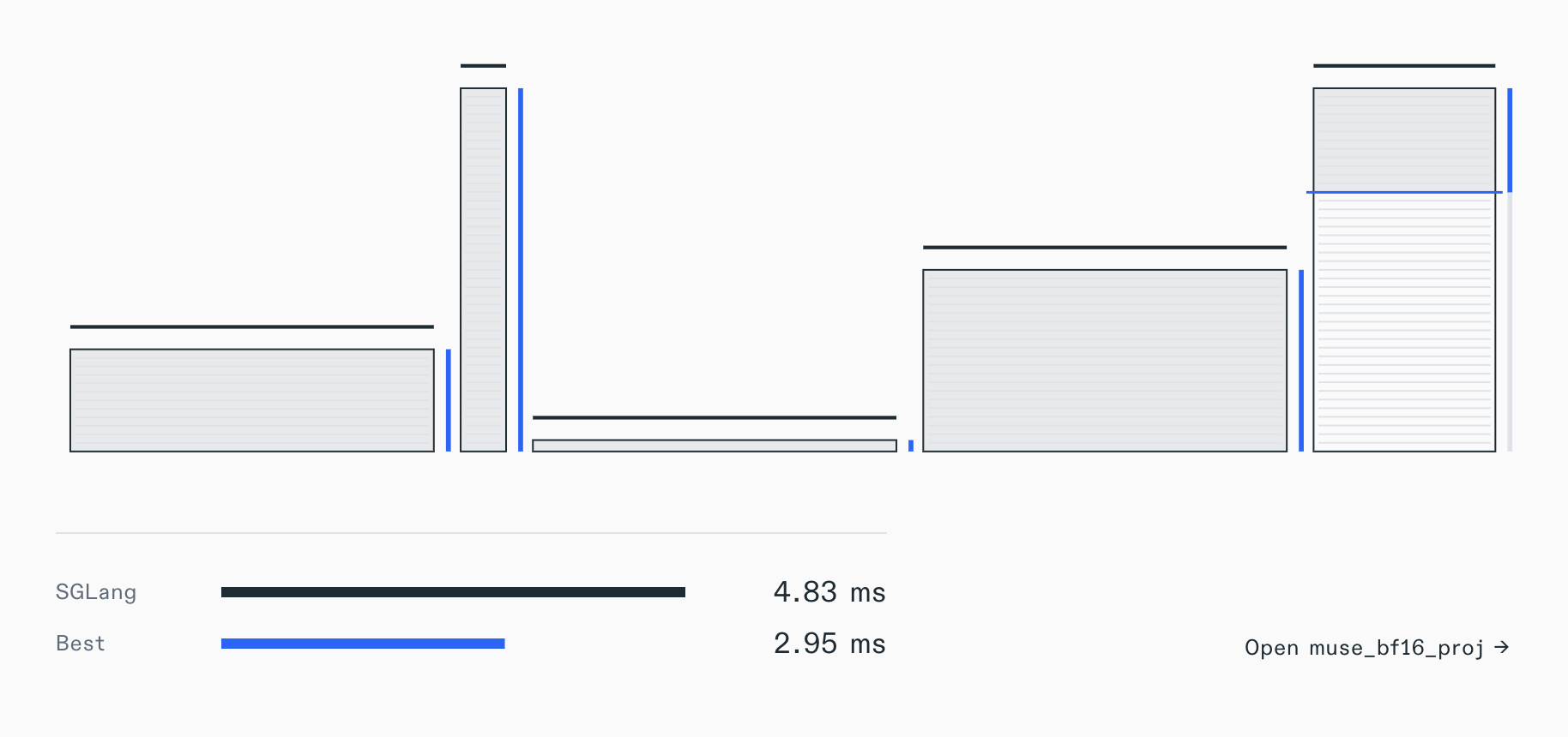
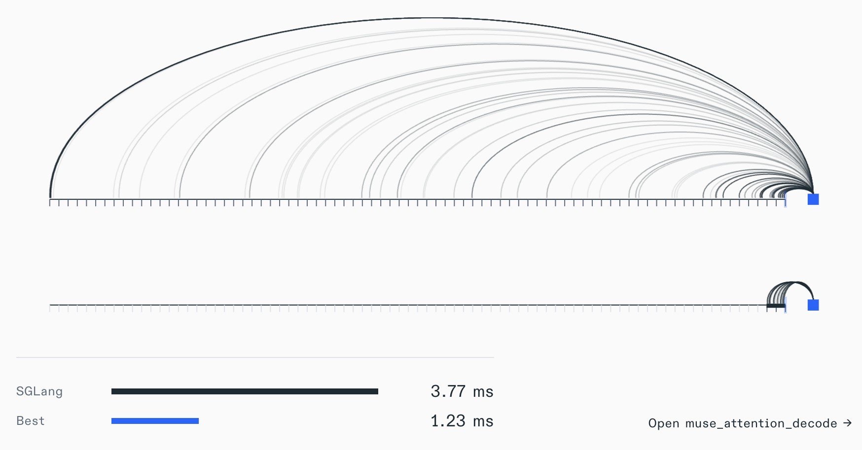
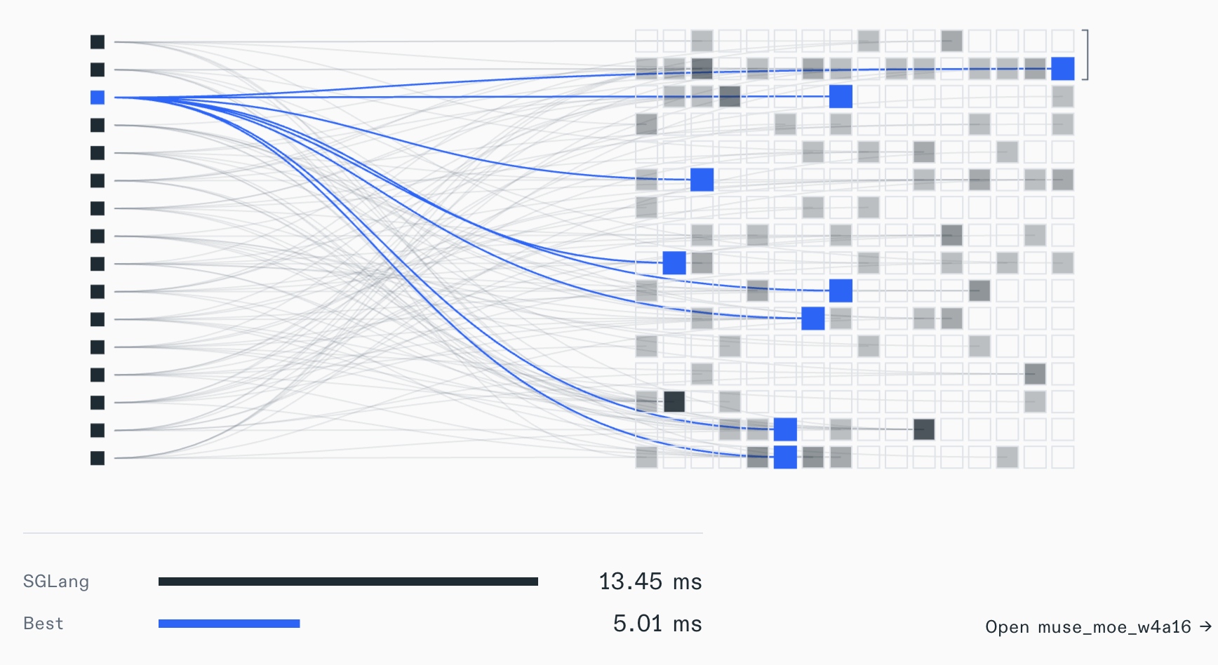
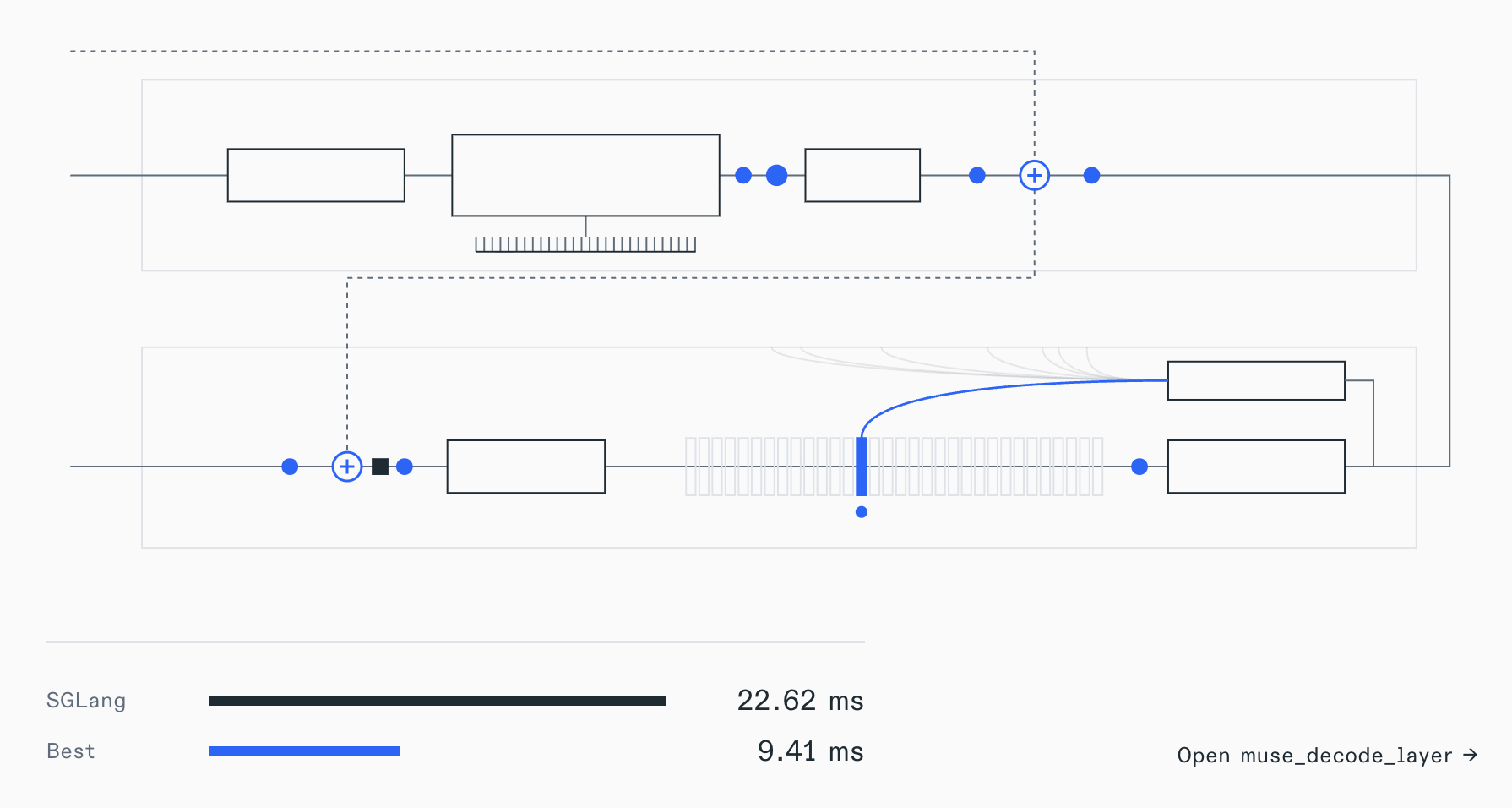
The pictures are the ones on the challenge’s site. Under each one, the two bars are SGLang’s time and the best submission’s, as they were on October 28.

Dense projections#

This problem is every plain matrix multiplication of the layer, the ones that aren’t attention or experts: $W_{qkvg}$ , $W_o$ , the router, and the two matrices that squeeze the token to 4,096 and bring it back to 8,192. They are in BF16, the router in FP32. With at most 256 tokens in a step, each weight is used at most 256 times every time it is read, so for most batches the time is just the time to read the matrices. This GPU’s part of $W_{qkvg}$ is 38 MB, and reading it at 4.8 TB/s takes about 8 µs, almost the same whether the step has 1 token or 128. SGLang takes 4.83 ms per step for all of them, and the best submission 2.95 ms.

Five matrices drawn to scale, with a line on top of each and a bar on its right — The five matrices one GPU holds, drawn to scale: the input runs along the top of each one and the output down its right side. From left to right, W_qkvg (8,192 in, 2,304 out: this GPU's q, k, v and g), W_o (1,024 in, 8,192 out), the router (8,192 in, 256 scores out, so thin it is almost a line), the squeeze (8,192 to 4,096) and the expand (4,096 to 8,192).

Attention while generating#

This problem starts at the output of $W_{qkvg}$ and ends at the output gate: QK-norm, RoPE in the sliding layers, writing the new $k$ and $v$ into the FP8 cache, attention, its norm and the gate. With one new token per conversation there is almost no math to do. The time goes into reading the cache: at 80K tokens, a full layer reads about 20 MB of it for every conversation, and a sliding layer, which only looks at the last 2,048 tokens, about 40 times less. SGLang takes 3.77 ms per step, and the best submission 1.23 ms.

A new token linked by arcs to all earlier tokens on top, and only to the last few below — The new token is the blue square on the right, and the tokens before it are the ticks on the line. Each arc is one earlier token it is compared with. On top a full layer, which reaches back over the whole context; below a sliding layer, which only reaches the last 2,048 tokens.

Routed experts#

This problem is the 32 experts of this GPU, between the squeeze and the expand: for each token and each of its picks that lives here, the gate, up and down matrices in NVFP4, the norm on the output, and the router’s weight before adding the 8 up. The routing is skewed so that this GPU is the busiest one, the case from when many tokens pick the same expert. With one token, only a few of its 8 picks land on this GPU. With 256 tokens, the experts in use get about 16 tokens each on average, below the 58 where the math starts to matter, so for most of them the time is reading their 4-bit weights. The routing also gives some experts many more tokens than others: the most popular one can get over 100. SGLang takes 13.45 ms per step, the most of the three pieces, and the best submission 5.01 ms.

Tokens on the left linked to experts in a 16 by 16 grid on the right — Tokens on the left and the 256 experts as a 16 × 16 grid on the right. Each token has a line to each of its 8 experts; one token's 8 are in blue, and the darker an expert, the more tokens picked it. The bracket on the top right marks the two rows this GPU holds, its 32 experts.

The whole layer while generating#

This problem is the three pieces above together, plus the norms and the two gates of the stream: one whole layer, from the stream that comes in to the stream that goes out. The communication between GPUs is left out, and each GPU acts as if the other seven had added nothing. SGLang takes 22.62 ms per step, close to the 22.05 ms of the three pieces added up, and the experts are more than half of it. The best submission takes 9.41 ms.

The layer as two rows of boxes joined by a dashed line — The layer in two rows, as in the overview of one layer. The top row is attention, from left to right: W_qkvg, attention over the FP8 cache (the ticks), its norm and the gate, W_o, a norm, ⊕ and a norm. The bottom row is the experts half and runs from right to left: the squeeze with the router above it, a norm, this GPU's 32 experts, the expand, a norm, ⊕ and a last norm. The blue dots are the norms and the gate, the ⊕ are where each half is added into the stream, and the dashed line is the stream going around them. The black square is the token going through. Of its 8 picks, one or two land on this GPU (lit), and the faint lines going up are the rest, going to other GPUs.

The whole layer while reading a prompt#

This problem is the same layer at the shapes of the experts section: a turn of 753 new tokens on an 80K-token conversation, four conversations at once, and the first turn in chunks of 16,384. Most of the time goes into the experts, as one large grouped multiplication over all of them. As in the roofline above, a single turn still waits on reading the weights, while four conversations at once and the first turn give the experts enough tokens for the math to matter. It has its own leaderboard, because reading a prompt is not part of a generation step. SGLang takes 387.4 ms for the whole set of cases, and the best submission 190.6 ms.

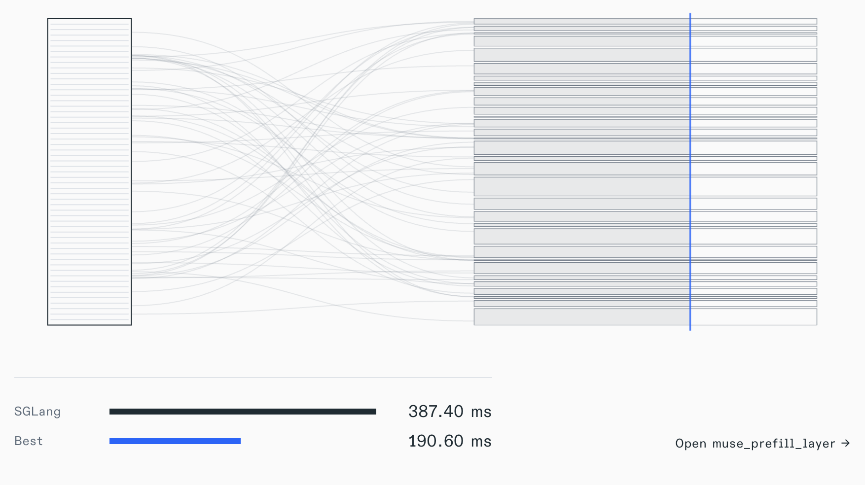
A tall block of tokens on the left linked to bars of different heights on the right — The 753 new tokens of a turn on the left. Their picks are sorted by expert into groups, one for each of this GPU's 32 experts, drawn as bars as tall as the number of tokens each one got. One grouped multiplication then runs over all of them: the blue line sweeping across.

The experts show up in three of the five problems, and in all three they are where most of the time goes.

Conclusion#

We’ve gone through the full Muse Spark Open architecture. We’ve seen how everything connects, and now the picture is crystal clear for tackling the 5 problems.

But answering one question left us with many more:

How do the 8 GPUs talk to each other?
How does this scale to millions of users?
What does each expert end up learning?
How do you train a router so the tokens spread evenly across the experts?

And I’m sure you have many more interesting ones of your own.

Thanks for reading :))